

Background
Electrical generation and transmission systems are generally sized to correspond to peak demand. To reduce peak demand or avoid system emergencies, we have two choices:
Add generation capabilities to meet the peak and occasional demand spikes
Add demand response (DR) program
Among these two choices, the DR is more cost-effective. The underlying objective of DR is to actively engage customers in modifying their consumption in response to pricing signals. On the appliance level, services of appliances are reduced according to a preplanned load scheme during the critical time frames.
Research Problem
To design a pricing scheme at the appliance level, we should know how users value the appliance. The research problem is: modeling the appliance level utility functions of users. To do this, we need to solve two problems:
Among all appliances, which appliance is more important to the user?
For certain appliances, how does the utility increase with the energy consumption?
Methodology
We will first introduce the dataset we use and then illustrate the utility model.
- Data Exploration
We use four data sources here as the independent variables for the model.
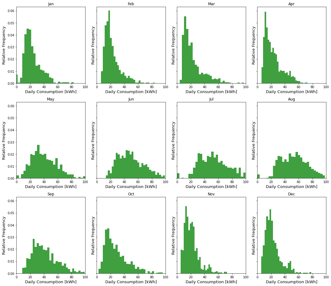
- Energy: average of the past week’s energy consumption associated with the appliance. An appliance like a dryer consumes more energy than other appliances and has a flatter distribution of energy consumption, while clothes washer, dishwasher, and microwave has low energy consumption.
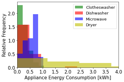 Histogram for energy consumption in a year
- Price: Tier price scheme according to the Austin energy department. The price increases when the accumulated energy consumption increases. The user in this case may considerably reduce the energy consumption to achieve a lower electricity bill.
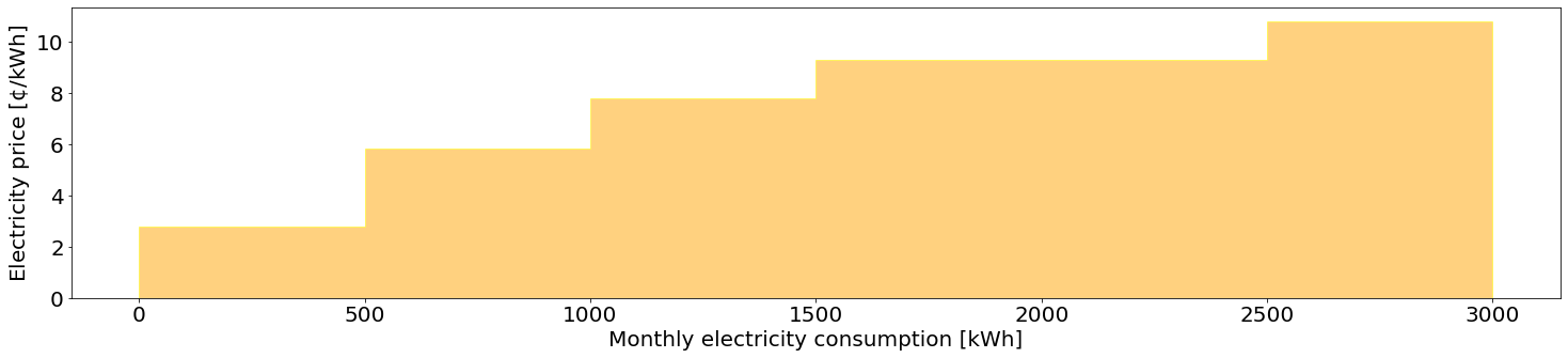 Tier price scheme for Austin
- Entropy: For each appliance, we convert energy consumption into a cumulative probability density function (CDF) and assign values to different CDF curve shapes using Shannon entropy.
In detail, for each appliance and each house, we extract the appliance energy consumption. We convert these counts into a cumulative probability density function (CDF). Our intuition is that the shapes of the CDF curves present useful information about how each house uses a specific appliance. For example, sharp jumps in a CDF mean that the residents use their appliances around specific values and would be less willing for shifting their usage. In contrast, the houses with smoother profiles would be more open to altering their original appliance usage schedule, as their usage times are more uniformly distributed across a day.
Next, we assign values to different CDF curve shapes, i.e., a function that translates a CDF curve into a numerical value. To achieve this, we use a well-known concept: Shannon entropy. Entropy is a measure of unpredictability of information content. In our case, when the appliance energy accumulates around certain intervals, the CDF curve has sharp jumps and becomes more predictable. Thus, the amount of information the CDF curve carries is low and this translates into low entropy. In contrast, a smoother CDF means that the appliance energy consumption is less predictable and thus it has a high entropy value.
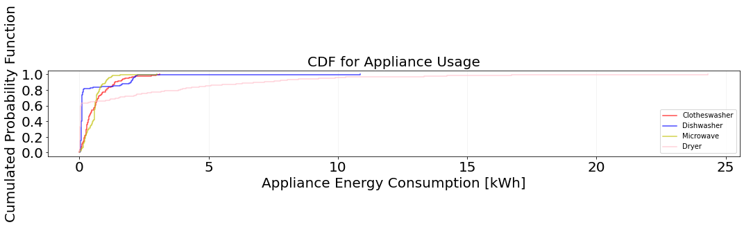 CDF for user’s appliance energy usage
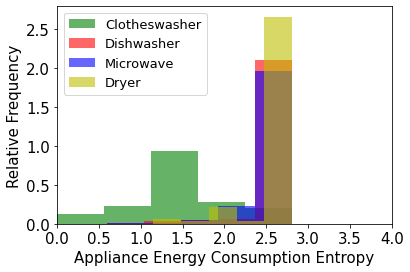 Histogram for entropy of user’s appliance energy usage
- Temperature: The temperature in Austin during a year, obtained through API. The temperature is higher from May to September, which leads to more energy consumption since people may use the air conditioning. Also, the temperature in summer fluctuates little compared to other months.
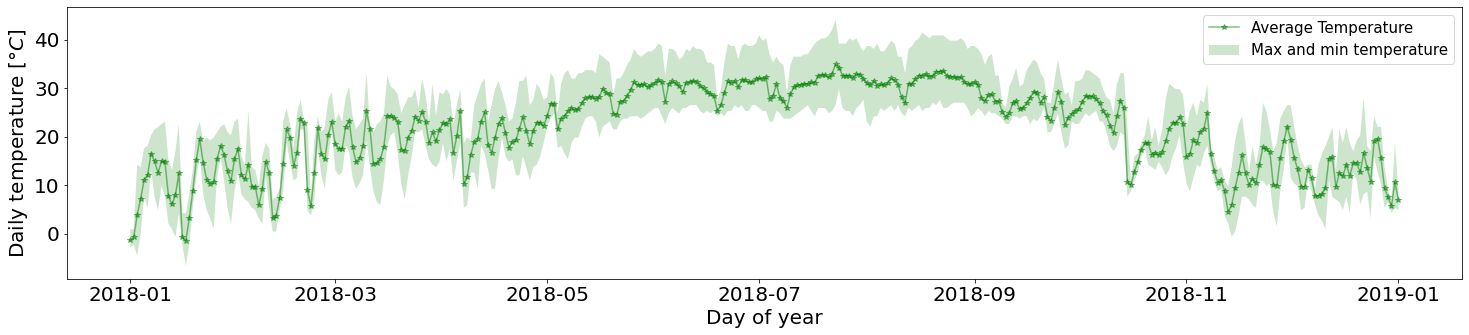 Daily temperature of a year
 Histogram for energy consumption in a year
- Utility Model
Which appliance is more important to the user?
- Discrete Choice Model to estimate the value of energy.
- Build the binary choice model.
- $U_{yes} = \beta_{0}+\beta_{energy} x_{energy} + \beta_{price} x_{price} + \beta_{entropy} x_{entropy} + \beta_{temperature} x_{temperature}$
- $U_{no} = 0$
- Estimate the parameters using Maximum Likelihood:
- $L* = \prod_{j=1}^{J} \prod_{i=1}^{I} P_{j}(i)y_{i,j}$
- $\hat{\beta} = \arg\max_{\beta} \ln L*(\beta_{e},\beta_{p},\beta_{r},\beta_{t})$
- Willingness to pay. coefficient of energy consumption/coefficient of energy price.
- $WTP = \frac{\partial price}{\partial energy} = \frac{\partial U/ \partial energy}{\partial U/ \partial price} = \frac{\beta_{energy}}{\beta_{price}}$
- Value of energy. willingness to pay * maximum energy consumption
- Build the binary choice model.
For certain appliances, how does the utility increase with the energy consumption?
- Quadratic Utility Function $U = ax(b-x)$.
- Rewrite as: $U = a’* (4/b^{2}) * x(b-x)$
- Scaler of the utility $a$: willness to pay for marginal increase in utility.
- Maximum energy consumption $b$: maximum energy consumption in past week.
Results
In this section, we first illustrate the estimation of the coefficients for the discrete choice model, and then we visualize the utility parameters of different users.
- Choice Model From the perspective of value, increases in entropy and temperature lead to a higher probability of using the appliance. Increases in consumption and electricity price lead to a lower probability of using the appliance. From the perspective of significance, the entropy and electricity price are significant while the consumption and temperature are not significant.
| variable | coef | std err | z | P>|z| | [0.025 | 0.975] |
|---|---|---|---|---|---|---|
| intersection | 0.3249 | 0.596 | 0.545 | 0.586 | -0.844 | 1.494 |
| entropy | 0.5904 | 0.236 | 2.503 | 0.012 | 0.128 | 1.053 |
| consumption, units:kWh | -2.6819 | 1.395 | -1.922 | 0.055 | -5.416 | 0.052 |
| electricity price, units:$/kWh | -12.6955 | 5.100 | -2.489 | 0.013 | -22.692 | -2.699 |
| temperature, units:C | 0.0169 | 0.016 | 1.027 | 0.305 | -0.015 | 0.049 |
- Utility Model The most important parameter in the utility model is the $a’$, which is also the willingness to pay. From the perspective of the mean value, the WTP is around 1 $/kWh, which makes sense. From the perspective of variance, the value is not very big for most appliances, except microwaves.
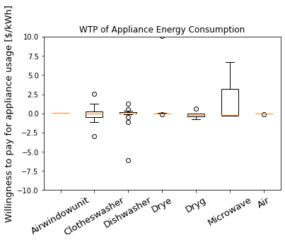 Willingness to pay for all users’ appliance
Conclusion
We have policy design insights from a qualitative perspective and a quantitative perspective.
Qualitative When designing the policy, we should consider the usage pattern of users (entropy and consumption). However, it is not enough. In mechanism design, the baseline of demand response is hard to estimate, since sometimes users will manipulate their historical data to show a false baseline, so as to obtain more benefits from the program. In this case, by estimating the willingness to pay for each appliance, it will be harder for the users to manipulate.
Quantitative With the utility function, the system operator can optimize the social welfare by plugging in the users’ utility values.
Reference
[1] Aksanli, Baris, and Tajana Simunic Rosing. “Human behavior aware energy management in residential cyber-physical systems.” IEEE Transactions on Emerging Topics in Computing 8.1 (2017): 45-57.
[2] Patnam, Bala Sai Kiran, and Naran M. Pindoriya. “Demand response in the consumer-Centric electricity market: Mathematical models and optimization problems.” Electric Power Systems Research 193 (2021): 106923.
[3] Brathwaite, T., & Walker, J. L. (2018). Asymmetric, closed-form, finite-parameter models of multinomial choice. Journal of Choice Modelling, 29, 78–112. https://doi.org/10.1016/j.jocm.2018.01.002